Last Updated: 2024-01-23
Background
If you've always wanted to learn SQL, this is the tutorial for you! It provides simple, easy-to-follow examples to get you up and running with SQL in no time.
Often, a drawback to learning SQL is the difficulty in finding an environment in which to practice. There is no need to worry about that in this case. Your Starburst Galaxy account comes equipped with sample data, so you'll be ready to go in no time.
Scope of tutorial
This tutorial uses Starburst Galaxy to teach you basic SQL techniques. It is designed both for beginners and those wanting to refresh their SQL knowledge. Special emphasis will be placed on understanding how SQL operates under real usage conditions.
Learning objectives
Once you've completed this tutorial, you will be able to:
- Query a dataset using basic SQL commands.
- Use SQL to join tables in a query.
- Use advanced SQL techniques to aggregate your query results.
Prerequisites
You need a Starburst Galaxy account to complete this tutorial. Please see Starburst Galaxy: Getting started for instructions on setting up a free account.
About Starburst tutorials
Starburst tutorials are designed to get you up and running quickly by providing bite-sized, hands-on educational resources. Each tutorial explores a single feature or topic through a series of guided, step-by-step instructions.
As you navigate through the tutorial you should follow along using your own Starburst Galaxy account. This will help consolidate the learning process by mixing theory and practice.
Background
What is SQL?
Structured Query Language (SQL) is a powerful and standardized language used in the management of relational databases, data warehouses, and data lakes. It serves as the foundational language for querying database management systems (DBMS) and is widely adopted across various platforms.
ANSI SQL
ANSI SQL is a standardized version of SQL that establishes the official features and syntax for SQL adopted by other dialects.
SQL Dialects
While ANSI SQL provides a common framework, it's important to note that different data systems may implement their own dialects, resulting in variations in syntax and functionality. Despite these differences, the fundamental principles of SQL remain consistent, enabling users to interact with and extract valuable insights from databases regardless of the specific dialect in use. Whether you're working with MySQL, PostgreSQL, or other relational database systems, understanding SQL empowers individuals to efficiently query, manipulate, and manage data.
Clusters vs catalogs vs schemas vs tables
Before you start using Starburst Galaxy to write SQL queries, it's essential to grasp three key terms: cluster, catalog, and schema.
Cluster
A cluster represents a collective of computational resources collaborating to process queries efficiently. You'll use a cluster when you enact a query in Starburst Galaxy.
Catalog
A catalog serves as a conduit to a data source. Catalogs come in many different types and configurations. For example, you might set up a cluster that accesses modern data lake storage technologies like AWS S3 or Azure ADLS, or more traditional data warehouses like Snowflake or Oracle. Catalogs unleash the power of Starburst Galaxy to connect to all of these data sources at once.
If you're interested in learning more about different catalog connections, we have a series of tutorials to walk you through the process step-by-step.
Schema
A schema delineates the organizational structure of data within a database. Schemas have a lot of use in Starburst Galaxy too and are one of the main building blocks of your data.
Table
Individual tables are the smallest component of this data architecture. They are used to structure relational databases in a system of columns and rows. They are a traditional data structure and have been the bedrock of Relational Database Management Systems (RDBMS) for decades.
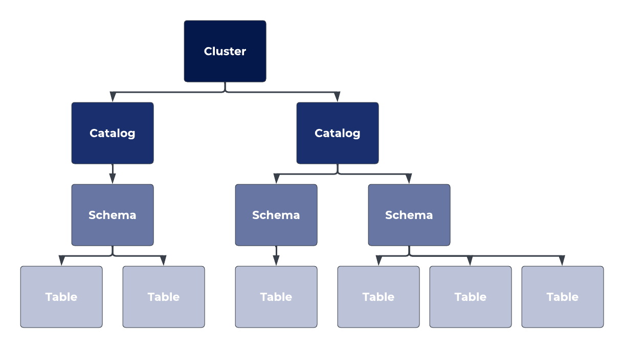
Hierarchical architecture
The relationship between these components is hierarchical. A cluster may encompass multiple catalogs, a catalog may encapsulate several schemas, and a schema may comprise multiple tables.
The image below depicts this relationship in more detail.
Background
Before we get started, it's time to set up the environment needed to run this tutorial.
This will make sure that you have the correct account, as well as the cluster, catalog, and schema needed to proceed further.
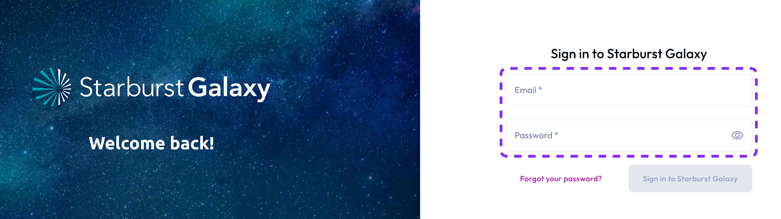
Step 1: Sign into Starburst Galaxy
The tutorial requires you to have a Starburst Galaxy account set up.
- Sign in to the account using the email associated with the account and password.
Step 2: Confirm cluster, catalog, and schema
When you sign in, you should see the cluster called free-cluster, sample catalog inside it, and demo schema inside that.
These are the cluster, catalog, and schema you will use for the SQL exercises in this tutorial.

Step 3: Setting the cluster, schema, and table
When you write a query, Starburst Galaxy needs to know which datasets you're accessing, and which schemas and tables you need.
Usually this means using the fully-qualified table name, which is written in a specific format:
You can think of this as the full name of the table. But just like a full name for a person, the fully-qualified table name is long. To avoid having to write this out each time, you can easily set the cluster, catalog, and schema for your session ahead of time and operate using shorter queries.
- In the query editor, select the appropriate Cluster, Catalog, and Schema using the drop down menus.
- Set Cluster to
free-cluster. - Set Catalog to
sample. - Set Schema to
demo.
Background
SQL has evolved from its origins in relational databases to become the preferred language for querying data across various sources. It is now employed in diverse environments, ranging from modern data lakes and data warehouses to traditional databases.
This section will show you how to use SQL to query a sample dataset, with a focus on data manipulation.
Step 1: Data Definition Language (DDL) vs Data Manipulation Language (DML)
SQL exists for many purposes. Overall, you can think of SQL being used for two distinct purposes:
- Data Definition Language (DDL)
- Data Manipulation Language (DML).
Data Definition Language
DDL operations create and define both structures and objects in a database and define the metadata within a DBMS. Some examples of DDL operations include CREATE TABLE, CREATE INDEX, ALTER TABLE, and DROP VIEW.
Data Manipulation Language
DML operations modify data within a database. These are the kinds of operations you will be using most in this tutorial. DML is used to manipulate data. Records , or rows, are created, modified, and accessed via DML. Some examples of DML operations are INSERT INTO table VALUES (‘val1', ‘val2', ‘val3'), SELECT...FROM...JOIN...WHERE.
Step 2: Understand SQL SELECT command syntax
Let's look more closely at an example of a DML command. The SELECT statement specifies the output of a SQL query. In its simplest form, it identifies both the table and columns to select data from. The data returned from the SELECT statement is called the result set.
The general syntax for a basic SELECT statement is:
SELECT column1, column2,...
FROM table_name;
Step 3: Select all records from a table
In the Starburst Galaxy query editor, it's time to view the data available for analysis in the astronauts table. This is one of the tables included in the sample dataset.
To do this, type the following query into the query editor and click the Run (limit 1000) button.
SELECT * FROM astronauts;Step 4: Use projection to query specific columns
Now, imagine that you wanted to read the same data, but only from specific columns. Selecting all of the data would be an inefficient way of doing that. Luckily, you can restrict the columns that are returned by your query.
To do this, you will need to specify the columns by name that you would like to include. This is called projection.
The example below shows projection in action. Notice that the column names are separated by commas:
SELECT
  name,
  nationality,
  mission_title,
  mission_number,
  hours_mission
FROM
  astronauts;
Step 5: Using the LIMIT and AS clauses
You can control the output of a query in a number of different ways. For instance, you can restrict the number of results returned using a LIMIT, or change the names of the results columns themselves to make them more meaningful or useful using the AS clause.
Limiting the number of results
Selecting all results works well, but it returns a lot of records. Sometimes, this might present a problem. Luckily, the LIMIT clause exists. It specifies the number of rows that you would like to return.
In the code below, this is set to 10.
Creating a column alias
You can also use the AS keyword to create an alias for each column.
Sometimes the existing column names are very long or aren't meaningful enough. Using AS is a simple way to set the column name in the results to something different.
This alias only exists for the duration of the query.
SELECT
    name AS full_name,
    nationality,
    mission_title,
    mission_number,
    hours_mission AS mission_duration
FROM
    astronauts
LIMIT 10;
Step 6: Understanding the WHERE clause
Imagine that you wanted to restrict the results of your query to ensure that only results that satisfy a given condition were returned.
This would be an example of conditionality, and would apply logical conditions to your search results. If a record fits those conditions, it will be returned; if it does not fit those conditions, it will not be returned.
To accomplish this, you should use the WHERE clause. The syntax for the command is shown below:
SELECT
    column1,
    column2, ...
FROM
    table_name
WHERE
    condition;
Step 7: Using the WHERE clause
It's time to try this out. The code below uses the WHERE clause to query the missions table and only return missions that are classified as a success.
SELECT
  company_name,
  status_rocket,
  cost,
  status_mission
FROM
  missions
WHERE
  status_mission = 'Success';
Step 8: Using wildcards and boolean logic
Using WHERE and NOT LIKE
Do you notice anything interesting? There are many astronauts from both the U.S. and U.S.S.R. You can use the WHERE clause in conjunction with the NOT LIKE operator to return only the astronauts from countries other than the U.S. or U.S.S.R.
Using wildcards
To do this, you'll also need to include a wildcard, which substitutes characters in a string. Two of the most common wildcards used with the LIKE (or NOT LIKE) operator are the percent sign (%) and underscore (_).
- The
%represents zero, one, or multiple characters. - The
_represents one single character.
Combining both methods
If you are trying to search for countries that are not the U.S. or U.S.S.R. which wildcard do you think is needed? Notice that both countries start with the letters "U.S.", but one has extra characters where the other does not. For this reason, the % wildcard is suitable.
Run the following query to see all of this in action:
SELECT
  name,
  nationality,
  mission_title,
  mission_number,
  hours_mission
FROM
  astronauts
WHERE
  nationality NOT LIKE 'U.S.%';
Step 9: Understanding how to use boolean operators
There are several operators that can be used in the WHERE clause. Use this table as your guide.
Operator | Description |
| greater than |
| less than |
| equal |
| greater than or equal |
| less than or equal |
| not equal |
| specifies the set of possible values |
| specifies a range of possible values |
| specifies a pattern |
Step 10: Using the ORDER BY clause
Imagine that you wanted to control the order in which results were displayed. To do this, you can use the ORDER BY clause to sort a result set by one or more output expressions. These results are returned in ascending order by default. To sort the records in descending order, use the DESC keyword, as shown in the example below.
It's time to test out this command.
- Use
ORDER BYto view the results of the previous query in descending order of nationality and name.
SELECT
  name,
  nationality,
  mission_title,
  mission_number,
  hours_mission
FROM
  astronauts
WHERE
  nationality NOT LIKE 'U.S.%'
ORDER BY
  nationality,
  name DESC;
Step 11: Using aggregate functions
Aggregate functions operate on a set of values to compute a single result.
Some examples are:
COUNT()- Returns the number of rows that satisfy a specific criterionAVG()- Returns the average value of a numeric columnSUM()- Returns the total sum of a numeric columnMAX()- Returns the largest value in a specified columnMIN()- Returns the smallest value in a specified column
In the following example, you'll use one query to find three different aggregate values: the number of trips, the longest mission in hours, and the smallest mission in hours from countries outside of the U.S. and U.S.S.R.
Run the query to see the results:
SELECT
  COUNT() as trips,
  MAX(hours_mission) as longest_mission,
  MIN(hours_mission) as shortest_mission
FROM
  astronauts
WHERE
  nationality NOT LIKE 'U.S.%';
Step 12: Using the GROUP BY command
The queries you've been using so far are great if you want to evaluate all the data together.
Now imagine that you want to increase the granularity level and evaluate the aggregates specifically for each country.
You can do this using the GROUP BY clause, which groups rows that have the same values into summary rows.
Try it out yourself using the code below.
SELECT
  nationality,
  COUNT() AS number_trips,
  MAX(hours_mission) AS longest_time,
  MIN(hours_mission) AS shortest_time
FROM
  astronauts
WHERE
  nationality NOT LIKE 'U.S.%'
GROUP BY
  nationality;
Step 13: Using the ORDER BY command
Next, you're going to change the query to restrict the order in which the results are returned.
Add an ORDER BY clause and sort the results by most trips per country. In the case of a tie, sort additionally by longest mission.
The result should resemble the code below.
SELECT
  nationality,
  COUNT() AS number_trips,
  MAX(hours_mission) AS longest_time,
  MIN(hours_mission) AS shortest_time
FROM
  astronauts
WHERE
  nationality NOT LIKE 'U.S.%'
GROUP BY
  nationality
ORDER BY
  number_trips DESC,
  longest_time DESC;
Step 14: Using the ORDER BY command
Time to try something new. Revisit the previous missions query, and add an aggregate function to determine who spent the most money on successful missions.
Order this query by the total highest cost using the code below.
SELECT
 company_name,
  SUM(cost),
  status_rocket
FROM
  missions
WHERE
  status_mission = 'Success'
GROUP BY
  company_name,
  status_rocket
ORDER BY
  SUM(cost) DESC;
Try it yourself
The following exercises will allow you to practice what you've just learned.
If you're stumped, the solutions are provided for you in the next section of this tutorial.
- Question 1:
What does the asterisk (*) do when used afterSELECT? - Question 2:
How many astronauts were born during or before the year 1930? - Question 3:
Who are the two oldest astronauts in the database? - Question 4:
Return the id, details, and cost for the 20 most expensive missions, in descending order. In case of ties, order by id as well. - Question 5:
Return a count of female astronauts. - Question 6:
This one will require some research on your part. How many companies are included in the missions table?
The following answers provide the solutions to the questions asked in the last section of this tutorial.
Use them to check your answers or unblock yourself if you're stuck.
Answer 1:
The * returns all columns from a table. To improve query performance, It is better practice to identify which columns you would like, rather than using the *.
Answer 2:
The answer is 70. To get this answer, run the following query:
SELECT
   name,
   year_of_birth
FROM
   astronauts
WHERE
   year_of_birth <= 1930
Answer 3:
The answer is Georgi Beregovoi and John H. Glenn Jr. To get this answer, you can run the following query:
SELECT
    name,
    year_of_birth
FROM
    astronauts
ORDER BY year_of_birth;
Answer 4:
The answer to Question 4 should use code similar to the following.
SELECT
    id,
    detail,
    cost
FROM
    missions
ORDER BY
    cost DESC,
    id DESC
LIMIT
    100;
Answer 4:
SELECT
    count()
FROM
    astronauts
WHERE
    sex = 'female';
Answer 6:
You can use the SELECT DISTINCT statement to get the information you need. The query should return 56 rows, indicating 56 distinct companies.
SELECT DISTINCT
    company_name
FROM
    missions;
Background
One of the most powerful uses of SQL is joins. Data is typically stored in multiple locations, and whether that means multiple tables, different schemas, or different data sources, connecting that data will usually require a join.
For Starburst Galaxy, joins are especially important because they allow you to federate your query across data residing in multiple storage locations. For example, you can join data from a data warehouse with data from a data lake. Although this data is housed in entirely different systems, you can access it as if it resided in a single system.
Excited? Let's begin exploring SQL joins.
Step 1: Review the types of SQL joins
A SQL JOIN clause is used to combine data from two or more tables based on a common field or column between them.
There are four basic types of joins that will be covered in this tutorial: INNER JOIN, LEFT JOIN, RIGHT JOIN, and FULL JOIN.
- An
(INNER) JOINreturns records that have matching values in both tables. - A
LEFT (OUTER) JOINreturns all records from the left table and the matched records from the right table, addingNULLfor missing matches on the right side. - A
RIGHT (OUTER) JOINreturns all records from the right table and the matched records from the left table, addingNULLfor missing matches on the left side. - A
FULL (OUTER) JOINcombines the results ofLEFT JOINandRIGHT JOIN. The results contain all rows from both tables, addingNULLfor missing matches on either side.
Step 2: Set up a tutorial environment
Now it's time to push further in your SQL journey with Starburst Galaxy.
In this section, you will use a different catalog and schema that are more suited to illustrating joins.
Understanding the tpch and tpcds datasets
The tpch and tpcds datasets are standard sample data used for benchmarking and testing. You can read more about the origin of these datasets and the specific data structures in the TPC documentation. Both datasets are included in Starburst Galaxy's standard sample dataset.
The tpch.sf1 schema contains the following tables: customer, lineitem, nation, orders, part, partsupp, region, and supplier.
- Set the catalog to
tpchand the schema tosf1.
Step 3: Using the INNER JOIN
An INNER JOIN selects records that have matching values in two tables. This type of join can be depicted in the Venn diagram below. For those familiar with set theory, an INNER JOIN is the intersection of the two tables.

The syntax for an INNER JOIN is:
SELECT
    column_name (s)
FROM
    table1
    INNER JOIN table2 ON table1.column_name = table2.column_name;
Step 4: Join the customer and orders tables
Let's take a look at this join in action using the customer and orders tables.
Suppose you wanted to join the customers and their orders from the two tables.
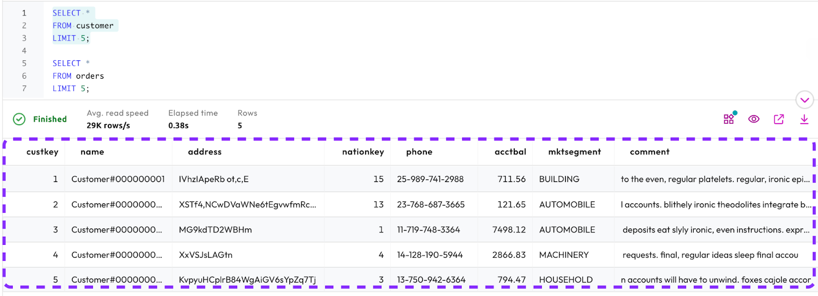
First, run the following query to take a look at the first five rows from each of these tables. Don't forget that the data is being generated dynamically, so some of the entries may look a bit strange.
SELECT *
FROM customer
LIMIT 5;

SELECT *
FROM orders
LIMIT 5;
Step 5: Select records from customer table
The output you return should look similar to the following.
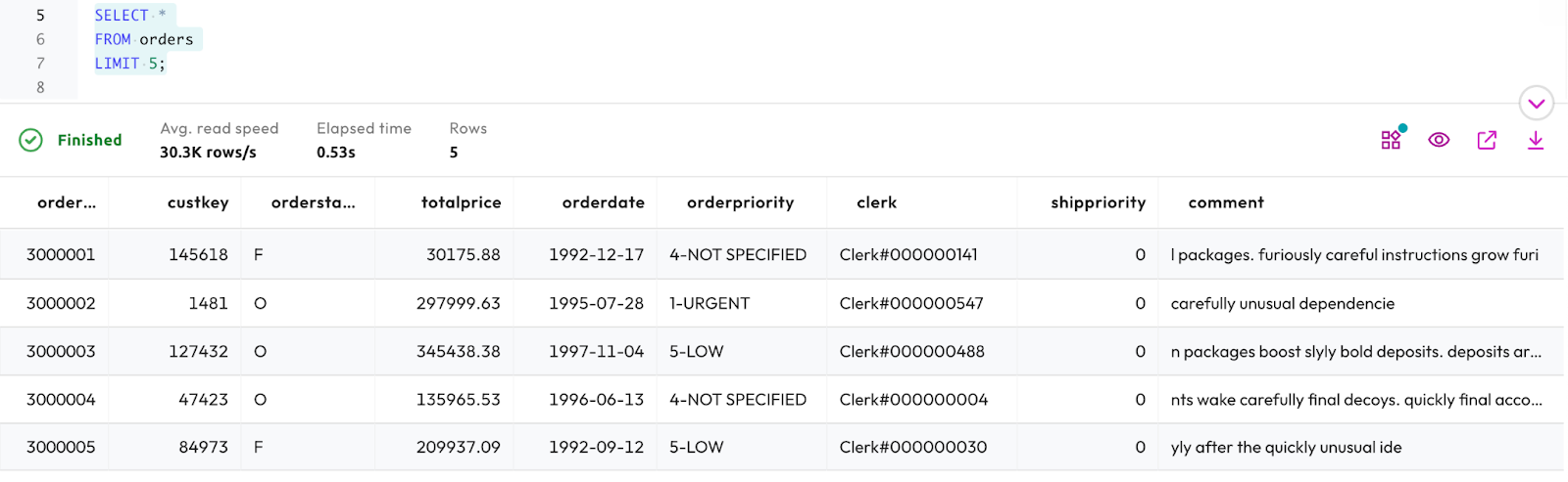
Step 6: Select records from order table
The output you return should look similar to the following.
Step 7: Join records from customer and order table using INNER JOIN
A quick glance at the two tables shows that custkey is the common column across both tables, so that can be used to join them.
Run the following query to try it out:
SELECT
    orders.orderkey,
    customer.name
FROM
    orders
INNER JOIN customer ON orders.custkey = customer.custkey;Step 8: Using the LEFT (OUTER) JOIN
A LEFT (OUTER) JOIN returns all records from the left table and the matched records from the right table. The left table is the first table that is listed in the query, while the right table is the second.
The syntax for a LEFT JOIN is:
SELECT
    column_name(s)
FROM
    table1
    LEFT JOIN table2 ON table1.column_name = table2.column_name;
The following Venn Diagram is a visual representation of a LEFT JOIN:
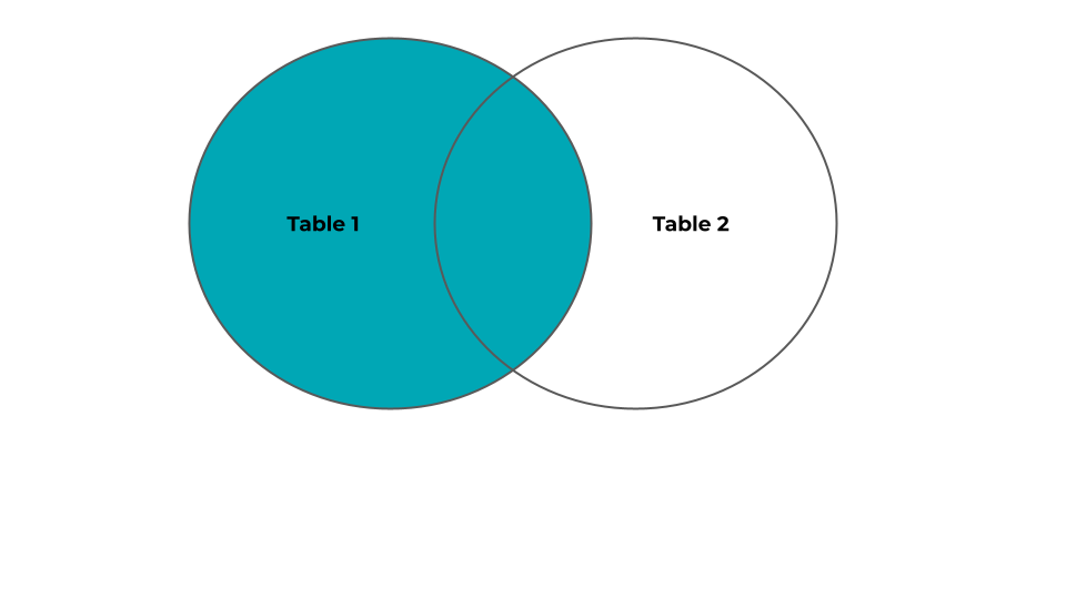
This example will look very similar to the one for an INNER JOIN. This time, the query will return all customers and any orders they might have, ordered by customer name. Because it is a LEFT JOIN, all records from the left table will be returned, even if there are no matching records on the right table. Run the following query to see the results:
SELECT
    customer.name,
    orders.orderkey
FROM
    customer
    LEFT JOIN orders ON customer.custkey = orders.custkey
ORDER BY
    customer.name;
Step 9: Using the RIGHT (OUTER) JOIN
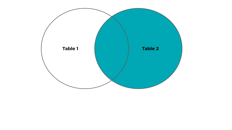
A RIGHT (OUTER) JOIN returns all records from the right table and the matched records from the left table.
The syntax for a RIGHT JOIN is:
SELECT
    column_name (s)
FROM
    table1
    RIGHT JOIN table2 ON table1.column_name = table2.column_name;
The following Venn Diagram is a visual representation of a RIGHT JOIN:
This example will utilize another table from the tpch.sf1 schema - the nations table.
Take a look at the first five rows of the table to get an idea of its composition:
nationkey | name | regionkey | comment |
0 | ALGERIA | 0 | haggle. carefully final deposits detect slyly agai |
1 | ARGENTINA | 1 | al foxes promise slyly according to the regular accounts. bold requests alon |
2 | BRAZIL | 1 | y alongside of the pending deposits. carefully special packages are about the ironic forges. slyly special |
3 | CANADA | 1 | eas hang ironic, silent packages. slyly regular packages are furiously over the tithes. fluffily bold |
18 | CHINA | 2 | c dependencies. furiously express notornis sleep slyly regular accounts. ideas sleep. depos |
Step 10: Using RIGHT JOIN on customer and nations tables
Notice that the nationkey column is also found in the customer table. Let's use that to join the customer and nations tables.
A RIGHT JOIN will return all customers and their nation of origin, if that information is available.
Run the following query to experiment with a RIGHT JOIN.
SELECT
    nation.name,
    customer.name
FROM
    nation
    RIGHT JOIN customer ON nation.nationkey = customer.nationkey
ORDER BY
    customer.name;
Step 11: Using the FULL (OUTER) JOIN
A FULL OUTER JOIN combines the results of a LEFT JOIN and RIGHT JOIN. In other words, it returns all records from both tables, regardless of whether there is a match.
The syntax for a full join is:
SELECT
    column_name (s)
FROM
    table1
    FULL OUTER JOIN table2 ON table1.column_name = table2.column_name;
The following Venn Diagram is a visual representation of a FULL JOIN:

Step 10: Using FULL (OUTER) JOIN on customer and nations tables
Now it's time to try out FULL (OUTER) JOIN on our dataset.
Run the following query to return the first twenty rows from the customer and orders tables, with or without matches.
SELECT
    customer.name,
    orders.orderkey
FROM
    customer
    FULL JOIN orders ON customer.custkey = orders.custkey
ORDER BY
    customer.name
LIMIT 20;
Try it yourself
The following exercises will allow you to practice what you've just learned.
If you're stumped, the solutions are provided for you in the next section of this tutorial.
- Question 1:
Would the results be different if you chosecustomeras table 1 andordersas table 2? - Question 2:
Re-run the following query to return the first twenty rows from thecustomerandorderstables. You ran it before during the tutorial. This time, you're going to look at it again to find out some new information.
Why is there aNULLvalue in theorderkeycolumn in the results set?
SELECT
    customer.name,
    orders.orderkey
FROM
    customer
    FULL JOIN orders ON customer.custkey = orders.custkey
ORDER BY
    customer.name
LIMIT 20;- Question 3:
Find all of the suppliers that are selling parts with a retail price of less than $920.
Hint: You'll need to join three tables for this one! - Question 4:
Retrieve the customer name and total number of orders for the customer withcustkey14.
The following answers provide the solutions to the questions asked in the last section of this tutorial.
Use them to check your answers or unblock yourself if you're stuck.
Answer 1
The results of the join would be the same, regardless of join order.
Answer 2
Because this is a FULL JOIN, all rows are returned, regardless of whether there are matches. The NULL value means that for that particular customer, there are no orders.
Answer 3
Use an INNER JOIN for this one, joining the part, partsupp, and supplier tables.
SELECT
    supplier.name AS supplier,
    part.name AS part,
    part.retailprice AS price
FROM
    part
    INNER JOIN partsupp ON part.partkey = partsupp.partkey
    INNER JOIN supplier ON partsupp.suppkey = supplier.suppkey
WHERE
    part.retailprice < 920
Answer 4
This is a LEFT JOIN, with orders as the left table.
SELECT
    customer.name,
    COUNT(orders.orderkey) AS order_count
FROM
    orders
    LEFT JOIN customer ON customer.custkey = orders.custkey
WHERE
    customer.custkey = 14
GROUP BY
    customer.name;
Tutorial complete
Congratulations! You have reached the end of this tutorial, and the end of this stage of your journey.
You have learned how Starburst Galaxy uses SQL to enact powerful queries, including different types of joins. Although all of the exercises in this tutorial focused on joining data within a single database, Starburst also allows you to easily combine data from multiple data lakes, data warehouses, and databases, even those that are non-relational. Check out some of our other tutorials for more information.
Continuous learning
At Starburst, we believe in continuous learning. This tutorial provides the foundation for further training available on this platform, and you can return to it as many times as you like. Future tutorials will make use of the concepts used here.
Next steps
Starburst has lots of other tutorials to help you get up and running quickly. Each one breaks down an individual problem and guides you to a solution using a step-by-step approach to learning.
Tutorials available
Visit the Tutorials section to view the full list of tutorials and keep moving forward on your journey!